


Rob DuMoulin, Information Architect Knowledge Based Solutions, Inc.
Published and Presented:
April 2000 - IOUGA-Live Conference and Expert Sessions
October 2000 - Oracle Open World 2000

Architecting Data Warehouses for Flexibility, Maintainability, and Performance
Introduction
Data Warehouse Data Base Administrators (DBAs), Data Administrators, Data Modelers, and System Architects all realize the difficulty of designing data warehouses for both data loading and query response performance. Unfortunately, these two optimization strategies are mutually exclusive. Normalized transaction-oriented systems may ensure data loading performance and data integrity but are inherently slower at performing analytical queries. On the other hand, de-normalization and warehouse index strategies improve query performance but incur the penalty during data loading. Even when a proper balance between load and query performance is achieved, you must consider how efficient the design will be as the data warehouse grows in size, complexity, and usage. To achieve perfect balance between query performance and an ever-shrinking maintenance window, both the DBA and Data Administrator must share a common understanding of the complete life cycle of warehouse information. This paper identifies warehouse business issues and provides design solutions that ensure continued performance, flexibility, and maintainability of your warehouse system. The paper also discusses subtleties of dimensional modeling, data migration issues, and tuning strategies. The overall design priority stressed is query performance. The challenge is to architect the data warehouse and loading procedures to offset performance penalties inherent to loading a de-normalized design. Identifying business requirements is critical to the success of a data warehouse project, but is out of the scope of this paper. It is assumed that a thorough business requirement analysis has been completed and that the granularity, source system mapping, and attribute definitions satisfy the business needs.
What's In An Architecture?
If asked the question “Which is better, On-Line Transaction Processing (OLTP) or On-Line Analytical Processing (OLAP),” would your response be “OLTP,” “OLAP,” “Neither,” or “Both”? The most accurate answer is all of the above, depending on your business perspective. OLTP and OLAP are each designed to support specific business requirements. OLTP systems record business transactions and are designed for data load performance and data integrity. OLAP systems are designed for reporting flexibility and query performance. Trying to design a single system to perform both roles is destined to fail.
OLAP architectures range from fully Relational OLAP (ROLAP) to fully Multi-dimensional OLAP(MOLAP). A Hybrid mix between ROLAP and MOLAP is called HOLAP. Of the three architectures, each has strengths, weaknesses, and scalability limitations that must be understood when determining the appropriate solution for business requirements. In general, ROLAP is suited for larger-scale data warehouses where rapid query response time is not required but large volumes of sparse data are expected. MOLAP is best suited for more focused data mart reporting where quick response time is critical to the business and levels of aggregation are restricted. HOLAP architecture can exist anywhere between the ROLAP and MOLAP architecture, depending on business requirements. The performance of HOLAP architecture depends on whether the requested information is among the pre-aggregated data or not. This paper focuses on the enterprise-scale data warehouse consisting of multiple OLTP systems feeding a ROLAP dimensional data warehouse. In this scenario, MOLAP, ROLAP, or HOLAP data marts can be created from the dimensional data warehouse to satisfy particular business needs. Be aware that choosing the wrong architecture for the right reporting requirements may lead to poor performance, inability to scale, or underachieving business objectives. Any of those situations can result in a failed data warehouse.
The Dimensional Model
The Dimensional Data Model was popularized in Ralph Kimball’s books The Data Warehouse Toolkit(John Wiley and Sons, Inc., 1996) and The Data Warehouse Lifecycle Toolkit (John Wiley and Sons, Inc., 1998) and many published articles. A dimensional model is a ROLAP data warehouse design that optimizes reporting flexibility and query performance. Fundamentally, the dimensional philosophy in this paper is based on the same modeling techniques written and taught by Kimball. This paper extends those modeling concepts to handle various business situations.
A dimensional data model reflects business processes rather than available business information. When you hear of data warehouses needing redesign because business systems change, those warehouses were designed around available business information and not to support business processes. Dimensional architecture separates attributes into either normalized Business Measurements (Facts) or de-normalized Analysis Qualifiers (Dimensions). Facts are grouped according to analytical value, business need, and level of aggregation. Examples of a “Point of Sale” Fact group would include Gross Sales, Units Sold, and Quantity on Hand. Dimension tables are typically groupings of descriptive attributes de-normalized to increase performance. Examples of Dimensions groups include Time, Customer, Store, and Product. Fact measurements can be constrained on any dimensional attributes and hierarchies, giving the warehouse flexibility. Since the growth and large volume occurs in Fact tables, additional space needed for de-normalized dimensions is usually insignificant. This architecture is referred to as a “Star Schema” because Dimension tables connect to centralized Fact tables much like points of a star. Stars, like the one shown in Figure 1, are scalable designs providing flexibility and drill-down capabilities that are inefficient in normalized designs. A Star derivation, called a snowflake, occurs when dimension attributes are normalized into parent-child tables. Snowflakes are often used when two indirectly related dimensions share attributes at different levels or when referential integrity is desired. Snowflakes are shown as three lookup tables left of the Store dimension in Figure 1. OLTP modeling instinct causes first-time dimensional modelers to either classify dimension attributes as facts or blindly normalize dimensions into snowflakes.
The primary reason to avoid snowflakes in data warehouses is query performance. Small-scale data warehouses may not notice decreased query performance; however, degradation increases dramatically as dimensions and snowflakes grow in size. During the design phase, it is critical to remember that implementing snowflakes to save space is hardly ever worth the performance penalty. The amount of space saved is not significant unless dimensions performance is affected due to dimension size. So when are snowflakes acceptable? The author recommends using a derivation of snowflakes whenever lookup code referential integrity (RI) is desired or whenever the text defining a lookup code is not available at load time. This derivation involves duplicating snowflake attributes within the dimension entity. These attributes are populated at load time so queries never need to join to the snowflake table, making query response times optimal. If the RI is validated during a data staging process, the integrity constraint between Dimension and snowflake may be removed. Be aware that some query tools use the RI constraint to automatically infer relationships. Removing the RI constraint disables this feature.
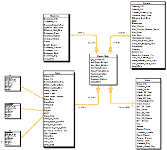 Figure 1. Star Schema with Snowflakes
If multiple dimensions reference a snowflake table, the snowflake should be maintained independently. Maintaining snowflake tables separately simplifies the load process of each referring “child” dimension because the stage records need only the snowflake key. The other extreme to maintaining snowflakes is to include all snowflake attributes within the dimension load record. The load process queries the snowflake for the exact permutation of its attributes. If the snowflake lookup determines an exact record does not exist, a new record is added to the snowflake and the attributes are entered into the dimension record. If the record is found, business rules determine how snowflake changes are handled. This second approach makes the snowflake self-maintaining, but you cannot enforce referential integrity of the load because a match is always guaranteed. The concept of using reference and self-maintaining tables is further discussed in this section.
The remainder of this paper refers to key fields within a data warehouse as either “Natural Keys” or “Warehouse Keys.” Source system primary keys are collectively referred to as the Natural Keys of the dimension. Natural Keys identify uniqueness in source system data at a specific point in time but are rarely primary keys in the warehouse because Natural Keys are not necessarily unique. Natural Keys can be combined with versions keys or effective dates to provide uniqueness. The more common approach is to use a sequence-generated Warehouse Key to represent the combination of Natural Key and version.
Kimball identifies three distinct types of dimensions (known by dimensional modelers as “Type One,” “Type Two,” and “Type Three”) that are based on how the dimension will represent history. Three other dimension types (“Profile,” “Lookup,” and “Reference”) are added toKimball’s dimension types to satisfy most business applications.
Type One Dimensions
Type One dimensions are applied to dimensional business entities where only the current state of the dimension is relevant. Changes to attributes in a Type One dimension are implemented as UPDATE statements, and no history is maintained. At first, business users may think that a Type One dimension fits their business model because they do not fully understand its consequences. Consider a historic report summarizing sales by month based on customer zip codes within a Type One customer dimension. Any report based on customer zip codes would be inconsistent every time a Type One customer changes postal regions. A report for January 1999 that is run in February 1999 may not report the same sales numbers as a January 1999 report run in September or even March 1999. Changing history is against the Laws of Physics and should be against the Laws of Data Warehousing unless specific business rules require it.
Type Two Dimensions
Type Two dimensions contain a separate record for distinct attribute combination of the Natural Key. All versions of a dimensional object are saved within the data warehouse by generating a sequential number (Warehouse Key) each time a new version of the Natural Key is added. This approach ensures that fact entries relate to time-consistent dimensional references. If dimensional properties change quickly over time, it may be necessary to separate dynamic attributes from more static ones (a possible candidate for Profile Dimensions, to be discussed later). The Natural Key allows all versions of an entity to be grouped together for analysis, if necessary.
Type Three Dimensions
Type Three dimensions handle changes by adding attributes within each record to indicate the previous, minimum, maximum, or original values (based on business rules). The limitation of this approach is the inability to reconstruct history and the loss of potentially valuable information when the versions exceed the fixed number of historical values. This author has never seen a pure business requirement for Type Three dimensions but has used a hybrid Type Two and Type Three approach simply to increase performance.
Profile Dimensions
Profile dimensions are simply Type Two dimensions in which all columns except the Warehouse Key are Natural Keys. This dimension type is typically used to group flags or finite-set attributes that classify or profile an object or state of an object. An example of a Profile dimension is eight single-character flags whose domain are “Y”, “N”, or NULL. The maximum number of records in this dimension would be 38, or 6,561. In reality, however, only a percentage of those permutations will be used. With a little coding, Profile dimension can be made self-sufficient by automatically populating entries only when asked for a combination not already in the dimension. If the maximum number is small or auto-loading is not an option, simply pre-populate the Profile dimension with all possible values prior to loading the data warehouse.
Lookup Dimensions
Lookup Dimensions contain attributes that represent static business characteristics. These dimensions do not have a business requirement to represent unknown or missing data conditions; thus, Natural Keys are usually the Lookup Dimension Primary Key. Such dimensions are typically small and static and won’t require an automated process to maintain them. Examples of lookup dimensions are state abbreviation codes supplied by the United States Postal Service or the names of Business Units within an organization.
Reference Dimensions
Reference Dimensions are similar to Lookup Dimensions, except they contain more records and may or may not be automatically maintained. These dimensions contain a Warehouse Key because they must represent “Missing” or “Invalid” dimensional entries. “Missing” and “Invalid” dimensional entries are used when fact records reference incomplete or incorrect information. An example of a Reference Dimension is a Calendar Dimension that is populated one time but must support error handling when source data is missing or corrupt.
Depending on loading and query requirements, several columns can be added to fact and dimension tables to improve flexibility and performance. All fact and dimension tables should reference an audit table containing the record entry and post date values that enable a data load to be backed out if necessary. Type Two dimensions should contain columns that define an effective begin and end timestamp, and a flag that identifies records as current or historical. Effective dating can be used to reconstruct the status or statuses of a dimensional entity over time. Remember that only the Warehouse Key is carried into a fact table. The Warehouse Key ensures that each fact record contains a time-consistent dimensional reference but in itself does not supply the state of a dimension at a specific point in time. To accomplish point-in-time analysis requires both an effective begin date and the end user to structure the query to return the maximum effective date that is less than a particular point in time. Providing both an effective begin and end date simplifies this process. Maintaining an indexed current-version indicator flag allows current versions to be identified without performing index range scan operations (an index on the Natural Key and current version flag is still not unique because there can be multiple records that are not current).
The last design consideration supports specific analyses without involving a fact table. This approach, called Dimensional Browsing, is available when all the information to answer a question resides within dimension tables. Consider a data model containing a Sales Representative and a Customer dimension with a need to support a business question such as:
How often are sales representatives responsible for customers outside of their district?
Answering this business question would involve joining the Customers and Sales Representatives dimensions through a sales fact table for unique sales representative and customer relationships, even though no fact-table attributes are needed. This analysis could be supported without involving the fact table by creating a combined (a.k.a. “Mini”) dimension of customer and sales representative attributes. While creating such a combined dimension must include the fact table, the query is performed only once (or each time the dimension is updated) and the Mini Dimension is much smaller because it contains only distinct combinations.
The Loading Process
The most challenging aspect of data warehouse development is loading data. Since business information typically exists on multiple non-integrated operational systems, information must be consolidated into a single point of record. The challenge lies in identifying the best source of record, standardizing codes and formats, handling data anomalies, and identifying data quality issues.
Flexibility
A fundamental concept that greatly simplifies data warehouse projects and ongoing maintenance is the use of data staging areas. Upon completion of the logical database design, data modelers have a good idea of the attributes and sources needed to populate the warehouse. At that time, a data staging area can be defined that serves as a dividing line between source systems and the warehouse. Stage should contain only the information needed to populate the warehouse and be organized to logically group information by type, not source system format. If a source record contains customer dimension and fact attributes, the source record should be split into two extracts instead of having a single stage table feed both the dimension and fact tables. Source system experts can begin to map the data in the source systems to this specification before the physical data warehouse is created. As the design becomes physical, warehouse architects map attributes from Stage to the production warehouse. Note that the two processes are performed independently of each other. This allows the source systems or the warehouse design to change without affecting processes or programs on the other side of the data stream.
Stage rarely contains indexes or constraints. Since the load processes from Stage are full table scans and the data presumably has integrity within the source system, indexes and constraints are unnecessary performance drains. Transformations occur during extraction and business rules are applied during the stage to the production warehouse load. Exceptions to these rules may exist, but the overall goal is to maximize data throughput.
Do not be tempted to pre-assign warehouse keys during source system extraction or stage area loading, as some keys may change based on load sequence. Dimension references from fact tables are time dependent. If dimension keys are assigned prior to fact table loading, any dimension table updates that occur prior to the fact load may invalidate the dimension.
Source system extracts should be written with the sole purpose of populating the Data Warehouse Stage area. Network traffic and the data-loading window can be significantly affected if extracts contain more rows or columns than necessary to satisfy stage requirements. The source system extract is also the most logical place to imbed business rules that apply only to a particular system. A gender code that is “M” or “F” in one system, “0” or “1” in another, and “Male” or “Female” in a third system should be standardized during each extract process. The Extract Specification document sets the standard format.
Maintainability
Standardizing load processes reduces the overall development and maintenance effort. Determine the business rules necessary to handle the consolidation, transformation, and loading of each warehouse table prior to implementation. Loading processes are similar for objects that possess the same functional qualities (like all Profile Dimensions).
Sequence-Generated Warehouse Keys are the primary keys of Type Two Slowly Changing
Dimensions and Profile Dimensions. The dimension loading process first checks if the Natural Keys exist in the dimension; the record is loaded if the Natural Keys are not found. If Natural Keys do
exist and any other record attribute changed (Type Two dimensions only), a new entry must be created to represent that record version. Finally, if the Natural Keys exist but no attributes have
changed, the record is a duplicate and is discarded. Figure 2 illustrates the Profile Dimension load process, and Figure 3 illustrates the Type Two Dimension load process.
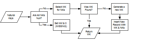 Figure 2. Profile Dimension Load Process
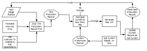 Figure 3. Type Two Dimension Load Process
Fact table loading is more straightforward than Dimension table loading. Staged fact table records are aware of dimension Natural Keys only, not dimension Warehouse Keys. Natural Keys for each Profile or Type Two dimension must be queried at load time to determine the correct Warehouse Key value. Figure 4 illustrates the fact table loading process.
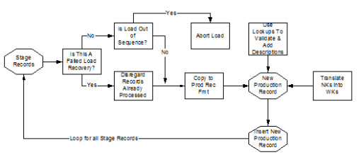 Figure 4. Fact Table Load Process
Loading Issues
Data quality of an OLTP system is typically as good as it needs to be, but hardly ever better. Even if source systems enforce referential integrity, they may not ensure the parent record is still a valid record. For example, over a 5-year period, a Distribution Center Clerk at a transportation company entered the same equipment code whenever products were moved around the facility. When history was loaded into a data warehouse, it became obvious that a single piece of equipment was responsible forall product movements for the past 5 years. The particular equipment was replaced 4.5 years before. When asked, the Distribution Center Clerk stated that the data entry screen accepted the default code so the clerk never had a reason to enter a correct one. This particular data quality issue made it impossible for that distribution center to analyze equipment maintenance trends. The data warehouse, however, was effective in identifying the data quality problem, and the data input screen was fixed within 2weeks.
One key issue that requires both a business decision and an implementation method is handling of missing or incomplete information. What happens if a sales record refers to an unknown customer or if the customer key is NULL? Remember that during a fact table load, the source-system fact record contains only the Natural Key for a customer (that is, SSN). The customer Natural Key must be converted to a customer Warehouse Key if the customer dimension is a Type Two slowly changing dimension. Missing and incorrect information is a symptom of two distinct problems, and each is handled differently. If the customer reference is not found in the customer dimension but is NOT NULL, then there are either data quality problems or a breakdown in the loading process. To the data warehouse, this customer is “Invalid.” If a NULL Customer Natural Key is passed in, this indicates that the source system did not provide a value. To the data warehouse, this customer is “Missing.”
If a dimension reference is deemed “Invalid” during fact table load, three options are available. The first and easiest approach is to discard the fact record. The advantage of this approach is ensuring only the highest-quality data exists in the warehouse. The disadvantage is that discarded records must be manually reprocessed and fact measures will not be included in the warehouse totals (at least initially). The second approach is to set the dimension reference to a specific dimension entry that indicates an “Invalid” dimension record. In this scenario, all fact records referring to invalid dimension entries are set to the same value and appear in a report as one group of “Invalid” entries. The advantage of this approach is that fact records are indeed loaded and a data quality percentage can easily be determined. The disadvantage of this approach is the inability to correct data once it is loaded because the Natural Key reference is lost (unless the load process outputs invalid Natural Key values). The third approach is inserting a new record into the dimension containing only the information that can be determined at load time (the Natural Key, the new Warehouse Key, a post date, and record creation date). While this approach always produces a valid reference and a loaded fact record, it may fill a dimension with trash data.
If a dimension reference is “Missing” during fact table load, only two options are available. The first option is to discard the fact record. The advantages and disadvantages are the same as if the dimension entry were “Invalid.” Another approach would be to set the dimension reference in the fact table record to a dimension entry that represents all missing records. This is the preferred approach because no information is lost in the assignment (the Natural Key was NULL) and the fact measures are loaded.
Data Load Recovery
An important aspect of automating the data load process is the ability to recover if one or more load processes do not complete. A requirement of recovery is a log of the production load process. Some of the basic attributes within a load log include job identifier, start time, end time, status, and last Natural Key committed. Records loaded, records failed, and duplicate record counters can provide loading metrics, if recorded.
Assuming the load failure was system-related and not due to data issues or error thresholds, two approaches perform recovery without the threat of data duplication. Small data warehouse loads can be contained within the rollback segment while other load processes are occurring and commit implicitly. When the load volume exceeds the rollback segment capacity, periodic commits are required. Sort larger loads by a Natural Key whose cardinality is sufficient to not fill the rollback segment and commit each time the key changes or by some increment of that key. Make sure all records of a key value are processed prior to a commit and record the last committed Natural Key value within the load log. At the start of each load, check the last load status and begin after the recorded last commit key if the previous load did not finish.
Performance
Data Warehouse Architects usually design systems to address specific analytical business needs. During the design process, the identified business questions form the measures and selection criteria of the front-end functional requirements. From this knowledge, it is easy to determine the strengths and weaknesses of the design. It is not likely that the warehouse will be at the exact level of granularity as all the queries run against it. Likewise, it is not likely that every business question involves one -- and only one -- fact table. To avoid the performance penalty of joining multiple fact tables or continually summarizing rows, use aggregation tables to satisfy reporting or combined fact table requirements. Queries needed to summarize information into aggregation tables can be optimized and the summary process can be done either as part of the data load process or by using materialized views (a.k.a. snapshots).
Data partitioning is a useful optimization tool that can dramatically reduce I/O when data access methods are predictable. Partitioning is also useful for archiving data that is no longer needed in the warehouse. To determine the best way to implement partitioning, you must first understand the data distribution, data access requirements, and how partitioning works. Partitioning physically segments rows based on the value of one or more key fields. The two algorithms available for determining how to distribute rows across available partitions are “Range” and “Hash” partitioning. Range partitioning sets minimum and maximum key values that can reside in a physical partition. This approach works well when data is distributed relatively evenly across key values. Time, for example, is a good candidate for a range partition key. Time-oriented data warehouses (billing, financial, sales, etc.) contain predictable fact table volumes when organized by time. A Range Partitioning strategy by time may group fact records based on month and year, resulting in 12 partitions per year. Archiving a month’s data would be as simple as taking a single partition off line and backing it to tape. Hash partitioning transparently assigns each partition key to a specific partition. When the distribution of the partition key is not predictable, choose the Hash Partition method to ensure a random distribution of rows across partitions. A random distribution, however, is not necessarily an even distribution. If a few keys contain the majority of information, then a few partitions will contain a majority of the rows. There is always the chance that one partition will contain almost all the rows, thus negating any benefit.
Queries that constrain on partition keys access only those partitions that meet the specific criteria. This ability to eliminate large segments of data from consideration is powerful if queries are written to take advantage of partition keys. One method to ensure that queries use partition keys is to create views for each partition or logical groups of partitions that automatically perform the proper constraining transparent to the user.
Because query performance is critical to a data warehouse, it is important to have an indexing and tuning strategy. The architecture and characteristics of data warehouses make it possible to generalize some rules concerning the initial indexes that should be created. Naturally, primary key indexes are necessary. Foreign key indexes in fact tables are beneficial when dimension primary keys drive the query. For example, if a time dimension is first used to supply a list of time warehouse keys for an analysis (say, all Wednesdays in the first calendar quarter of a year), those key values are located in the fact table by the Foreign Key Index. Another frequently encountered query is identifying the Warehouse Key for a dimension row given its Natural Keys. This query must be done each time Natural Keys in the stage fact table are translated into Warehouse Keys during the load process. By creating an index containing all of a dimension’s Natural Keys, the revision identifier, and the Warehouse Key, this lookup can be performed solely within the index. Loading time is improved because the table is never accessed.
Profile dimension attributes that have a low cardinality are prime candidates for bit-mapped indexes that use binary arithmetic to resolve matches. Since Profile dimension lookups are based on all Natural Keys at load time, a bit-mapped index can be incredibly fast. Placing bit-mapped indexes on individual low-cardinality columns of a Profile dimension boosts performance on queries constraining on single Natural Keys. Bit-mapped indexes are also ideal for Profile dimensions because they provide indexing of NULL values. Beware of bit-mapped indexes during load time because the overhead to maintain them during large data loads is costly. Instead, drop bit-mapped indexes prior to a load and rebuild them after a load if the load will add any new distinct values to the columns.
Remember, data warehouse information is rarely updated or deleted. This characteristic allows the DBA to reduce the amount of free space left in data blocks to avoid row chaining. As a rule, leave the PCT FREE at 10 percent during development. Reduce the value for PCT FREE to 0 percent for known static dimensions (i.e. calendar), 2 to 4 percent for dimensions whose current record or effective dates are updated, and 0 percent for stage and fact tables (unless you require pre-processing or post-load processing that perform UPDATEs).
On occasion, you may determine that certain important queries take an excessive amount of time to return results. Besides verifying the correct execution plan or updating the statistics, consider reorganizing the rows within the data table to minimize the number of blocks returned during queries. Space and time permitting, you can do this by performing a CREAT TABLE … SELECT command by ordering the selected rows by the same criteria as the slow-performing query. Simply swap table names around and apply the indexes and constraints to the newly organized table. Because this may negatively impact performance of other queries, use this option sparingly. Even though this operation is viable only on manageable dimensions or fact table partitions, it can significantly reduce the number of physical reads.
Summary
The methods discussed in this paper apply to data warehouses of any business type. However, keep in mind that data warehouse requirements change as businesses change and good data warehouses can invoke rapid business changes. A simple design based on a business-oriented model is far more flexible than one that attempts to reproduce complex source-system data transformations. Strive to let the data warehouse identify data problems rather than correct them at load time.